Introduction
Urban transit networks are often discussed in terms of routes, schedules, and service frequency, but underneath those operational details sits a more fundamental question: how resilient is the network’s connectivity structure when links fail? A transit system can appear robust during normal operation while still depending heavily on a small set of corridors and transfer connections. When those critical links are disrupted—through construction, extreme weather, vehicle shortages, signal failures, incidents, or planned service cuts—the network may not simply get “slower.” It can fragment, producing sudden pockets of isolation where entire neighborhoods become difficult or impossible to reach by transit.
This project studies resilience from a network-science perspective using only Metro Transit General Transit Feed Specification (GTFS) schedule data, treating the transit system as a directed graph where nodes are stops and edges represent consecutive stop-to-stop movements within scheduled trips. Rather than analyzing any single disruption event, we simulate a broad class of disruptions by progressively removing edges from the graph and measuring how rapidly the system loses the ability to connect origin–destination pairs. This framing captures two distinct failure modes that matter to riders and planners:
- Connectivity collapse: trips become impossible because the network breaks into disconnected components.
- Efficiency degradation: trips remain possible, but detours and transfer burdens inflate travel costs dramatically.
A key theme of resilience research is that random failures and targeted attacks can produce radically different outcomes. Random failures approximate “everyday” disruptions—minor route segments lost due to localized issues. Targeted removals approximate adversarial or worst-case conditions—removing links that are structurally central or that carry a large share of flows, such as major downtown feeders, river crossings, or transfer bottlenecks. In transit terms, targeted disruptions resemble the loss of a high-impact corridor or a cluster of interdependent connections that triggers cascading rerouting pressure elsewhere in the system.
To make these comparisons concrete, we evaluate five edge-removal strategies. One represents random failures via Monte Carlo simulation. The remaining strategies represent targeted attacks and vary along two dimensions: static vs. adaptive and weighted vs. unweighted. Static targeted removals use a fixed precomputed ranking of “critical” edges from the baseline network; adaptive strategies recompute edge importance after each removal to mimic a compounding cascade where the next failure strikes whatever has become newly load-bearing. Weighted variants incorporate a generalized travel-cost perspective (capturing both in-vehicle time and frequency-related waiting penalties), while unweighted variants focus on pure topology. Together, these strategies span a spectrum from benign disruptions to worst-case, system-seeking failures.
Because transit service is not uniform across time, resilience can also depend strongly on when disruptions occur. The same city can behave like four different networks depending on service patterns: dense weekday service, sparse weekend service, and peak-period service that concentrates capacity along commuter corridors. Accordingly, we build four scenario-specific GTFS graphs—weekday, weekend, AM peak, and PM peak—and run the same disruption experiments on each. This allows us to quantify how redundancy changes with service levels and how that redundancy moderates (or fails to moderate) network collapse.
The contributions of this project are threefold:
- A GTFS-only resilience framework that requires no ridership counts, external demand models, or GIS layers, making it portable across agencies that publish GTFS feeds.
- A multi-strategy disruption comparison that separates random failure behavior from targeted and cascade-like degradation, clarifying how “robustness” depends on the nature of disruption.
- Scenario-specific insights showing how resilience shifts across weekday, weekend, and peak service patterns—highlighting the structural consequences of reduced redundancy.
Ultimately, the goal is not to predict the next disruption event, but to identify the network features that function as load-bearing elements. If a small number of links disproportionately control connectivity, they become prime candidates for resilience planning: operational contingencies, redundancy investments, or service design changes that reduce single points of failure. By quantifying how quickly connectivity and travel cost deteriorate under different disruption models, this study provides a structured way to discuss transit resilience in terms that are both measurable and actionable.
The baseline network structure is easiest to understand visually: Map 1 shows the full GTFS-derived network before any removals, where the densest bundles of overlapping segments concentrate in the urban core and along major cross-river and downtown approach corridors. Those dark, repeated alignments mark baseline corridors that carry a large share of shortest paths, so static targeted removals hit them early. But because the downtown core has many alternative routes, the network ofter reroutes around these losses; adaptive strategies become most damaging when recomputed centrality shifts attention to newly exposed bridge-like connectors outside the redundant core, accelerating fragmentation.
Methods
This project measures the structural resilience of a public transit network using GTFS-only data. We construct scenario-specific directed graphs (weekday, weekend, AM peak, PM peak), remove edges progressively under several disruption strategies, and quantify how network connectivity and effective travel cost degrade as disruptions accumulate.
Data Source and Inputs (GTFS)
All analysis is derived from the static GTFS feed files:
stops.txt— stop IDs and coordinates (lat/lon)trips.txt— trip-to-route metadata andservice_idstop_times.txt— ordered stop sequences and times per tripcalendar.txt(optionallycalendar_dates.txt) — service patterns by weekday/weekendshapes.txt— polyline geometry used for map rendering (not required for analysis)
No external ridership, census, roadway, or schedule-reliability data is used. The network structure and weights are inferred from GTFS schedules alone.
Scenario Definitions
We build four scenario graphs by filtering trips using GTFS service calendars and trip start times.
Weekday service (baseline all-day)
A service_id is classified as “weekday” if it operates on Monday–Friday and not Saturday/Sunday:
- monday=tuesday=wednesday=thursday=friday = 1
- saturday=sunday = 0
All trips with those service_ids are included.
Weekend service
A service_id is classified as “weekend” if it operates on Saturday or Sunday:
- saturday=1 OR sunday=1
All trips with those service_ids are included.
AM Peak and PM Peak (weekday only)
Peak scenarios start from the weekday trip set, then keep trips whose first stop’s departure time lies in a time window:
- AM Peak: first departure in [06:00:00, 09:00:00)
- PM Peak: first departure in [15:00:00, 18:00:00)
This yields two “peak-only” subnetworks that represent commuter-oriented service patterns.
Time Parsing and Cleaning
GTFS allows times beyond 24:00:00 (e.g., 25:13:00). Times are parsed to “seconds since midnight” using:
sec = 3600*h + 60*m + s
For edge travel times computed from consecutive stops:
- Negative or non-finite values are treated as missing (
NaN) - Medians are computed using available valid samples
This step avoids invalid travel-time artifacts and ensures stable edge costs.
Graph Construction
Directed edges from stop sequences
For each scenario, we build a directed graph G = (V, E):
- Nodes
V:stop_id - Directed edges
E: consecutive stop pairs(u → v)appearing in any trip in the scenario
Edges are derived by sorting stop_times by (trip_id, stop_sequence) and taking the next stop in each trip.
Edge frequency (freq)
Each directed edge is assigned:
freq(u→v): number of distinct trips that traverse that edge in the scenario
Within a trip, repeated occurrences of the same (u→v) are de-duplicated so frequency reflects “trips using the edge,” not raw stop_time rows.
Edge in-vehicle travel time (time_med)
Each directed edge is also assigned:
time_med(u→v): median of(arrival_time at v) − (departure_time at u)across all trips using the edge (seconds)
The median is used for robustness to occasional schedule anomalies.
Generalized Edge Weight (w_gen)
To represent a GTFS-only notion of “effective travel cost,” we use a generalized edge weight:
- In-vehicle component:
time_med(u→v) - Waiting component (expected wait): derived from service frequency
Conceptually:
w_gen(u→v) = time_med(u→v) + E[wait(u→v)]
Where E[wait] is estimated using the common transit approximation:
- expected wait ≈ ½ × headway
And headway is inferred from scenario-level frequency (higher frequency → lower expected wait). This yields a cost that penalizes infrequent corridors even if their in-vehicle time is short.
Note: The visualization code can route edges along shapes, but the analysis weight is computed from GTFS schedules and edge frequency, not from geographic distance.
Edge Importance (Betweenness Centrality)
To identify “critical” links, we compute edge betweenness centrality (EBC) on each scenario graph. EBC measures how often an edge lies on shortest paths, making it a natural proxy for corridors that connect many origin–destination flows.
Weighted vs unweighted importance
We compute two EBC variants:
- Weighted EBC: shortest paths weighted by
w_gen(importance reflects effective travel cost) - Unweighted EBC: shortest paths ignore weights (importance reflects topology only)
Approximate computation
For scalability, EBC is approximated using n_sources sampled source nodes (NetworkX’s approximation):
- n_sources = 800 (configurable)
- fixed random seed for reproducibility
normalized=True
This produces a stable ranking of edges without the full O(|V||E|) exact computation.
To make the EBC ranking interpretable, we also extract the top 10 edges per scenario (directed stop-to-stop links) by weighted EBC. These edges represent the most “load-bearing” connections in the schedule-derived network under each service pattern. Notably, the highest-ranked edges repeatedly fall within the downtown core (e.g., Hennepin / 7th / Marquette segments), while weekend service exhibits larger peak EBC values—consistent with reduced redundancy concentrating shortest-path flow on fewer connectors. Peak-period networks also surface scenario-specific corridors (e.g., Central Ave ↔ University Ave in AM peak).
| u_name | v_name | edge_betweenness |
|---|---|---|
| Hennepin & 5th St Station | Hennepin & 4th St Station | 0.019279 |
| 7th St & 3rd/4th Ave Station | 7th St & Nicollet Station | 0.014655 |
| 7th St & Park Station | 7th St & 3rd/4th Ave Station | 0.014443 |
| Marquette Ave & 5th St - Stop Group B | Marquette Ave & 7th St - Stop Group B | 0.014135 |
| Marquette Ave & 7th St - Stop Group B | Marquette Ave & 9th St - Stop Group B | 0.014124 |
| Marquette Ave & 9th St - Stop Group B | 11th St S & Marquette Ave | 0.013844 |
| 7th St & Nicollet Station | 7th St & Hennepin Station | 0.012848 |
| 2nd Ave S & 5th St - Stop Group F | 2nd Ave S & Washington Ave S | 0.012038 |
| 2nd Ave S & 11th St - Stop Group F | 2nd Ave S & 7th St - Stop Group F | 0.011721 |
| 2nd Ave S & 7th St - Stop Group F | 2nd Ave S & 5th St - Stop Group F | 0.011711 |
| u_name | v_name | edge_betweenness |
|---|---|---|
| Hennepin & 5th St Station | Hennepin & 4th St Station | 0.031369 |
| 7th St & Park Station | 7th St & 3rd/4th Ave Station | 0.028542 |
| 7th St & 3rd/4th Ave Station | 7th St & Nicollet Station | 0.028524 |
| 7th St & Nicollet Station | 7th St & Hennepin Station | 0.028409 |
| 6th St & Minnesota Station | 6th St & Washington Station | 0.026984 |
| Wall St & 7th St / 6th St | 6th St & Jackson Station | 0.026869 |
| 6th St & Jackson Station | 6th St & Minnesota Station | 0.026851 |
| 6th St & Washington Station | 6th St & Washington St / 7th St | 0.021158 |
| 5th St & Minnesota St | 5th St & Jackson St | 0.018098 |
| 5th St & Jackson St | Wacouta St & 5th St / 6th St | 0.018079 |
| u_name | v_name | edge_betweenness |
|---|---|---|
| 7th St & Nicollet Station | 7th St & Hennepin Station | 0.015846 |
| Central Ave & 4th St SE | Central Ave & University Ave | 0.013995 |
| Central Ave & University Ave | Central Ave & 2nd St SE | 0.013982 |
| 7th St & 3rd/4th Ave Station | 7th St & Nicollet Station | 0.013747 |
| 2nd Ave S & 11th St - Stop Group F | 2nd Ave S & 9th St - Stop Group F | 0.013163 |
| 2nd Ave S & 9th St - Stop Group F | 2nd Ave S & 7th St - Stop Group F | 0.013151 |
| 2nd Ave S & 7th St - Stop Group F | 2nd Ave S & 5th St - Stop Group F | 0.013138 |
| 2nd Ave S & 5th St - Stop Group F | 2nd Ave S & Washington Ave S | 0.013126 |
| Hennepin & Gateway Station | Hennepin & 3rd St Station | 0.012799 |
| Hennepin & 3rd St Station | Hennepin & 5th St Station | 0.012786 |
| u_name | v_name | edge_betweenness |
|---|---|---|
| Hennepin & 5th St Station | Hennepin & 4th St Station | 0.026097 |
| 7th St & Park Station | 7th St & 3rd/4th Ave Station | 0.017987 |
| 7th St & 3rd/4th Ave Station | 7th St & Nicollet Station | 0.017969 |
| Marquette Ave & 5th St - Stop Group B | Marquette Ave & 7th St - Stop Group B | 0.015685 |
| Marquette Ave & 7th St - Stop Group B | Marquette Ave & 9th St - Stop Group B | 0.015673 |
| 6th St & Jackson Station | 6th St & Minnesota Station | 0.014130 |
| 6th St & Minnesota Station | 6th St & Washington Station | 0.014118 |
| Wall St & 7th St / 6th St | 6th St & Jackson Station | 0.014018 |
| 7th St & Nicollet Station | Hennepin & 5th St Station | 0.013892 |
| 7th St & Nicollet Station | 7th St & Hennepin Station | 0.013538 |
Disruption Strategies (Edge Removal Orders)
We simulate progressive disruptions by removing edges in a specific order. Five strategies are evaluated:
1) Random failure (Monte Carlo)
Edges are removed in a random order.
- repeated over many trials (e.g., 100)
- each trial uses a different RNG seed
- results summarized by the mean and 10th–90th percentile band
2) Static targeted (weighted)
Compute weighted EBC once on the original graph and remove edges from highest to lowest EBC.
- ranking does not change as the graph degrades
3) Static targeted (unweighted)
Compute unweighted EBC once and remove edges from highest to lowest EBC.
4) Adaptive targeted (weighted)
Repeatedly recompute weighted EBC after removals and always remove the currently most central edge.
- approximates an intelligent adversary / cascading failure
5) Adaptive targeted (unweighted)
Same as above but recomputing unweighted EBC after each removal.
Progressive Removal Schedule
For each scenario and strategy, we remove edges in increasing increments:
k ∈ {0, 10, 25, 50, 100, 200, 400, 800}
These values correspond to roughly 8–12% of edges in typical scenario graphs, depending on scenario density.
Baseline Node Set and OD Pair Sampling
To compare strategies fairly, all evaluations use a consistent baseline:
- Construct the baseline scenario graph
G0 - Compute its largest weakly connected component (LWCC)
- Sample origin–destination (OD) pairs only from nodes in the baseline LWCC
- Fix the sampled OD set once and reuse it for all
kand all strategies
This prevents comparisons from being distorted by changes in which nodes “exist” or are connected under different disruption sequences.
Shortest-Path Evaluation
At each removal level k, we build the post-removal graph Gk and evaluate shortest paths over the fixed OD sample:
- shortest paths computed using Dijkstra on
w_gen - distances are computed efficiently using repeated single-source shortest path runs
Two distance summaries are tracked:
Conditional on reachability (reachable-only)
Average shortest-path cost among OD pairs that remain connected at k.
This isolates efficiency degradation among surviving trips.
Penalized average (reachable + unreachable)
To keep averages comparable as connectivity collapses, unreachable OD pairs are assigned a large fixed penalty distance. The reported metric is:
- penalized path length ratio = (mean penalized distance at
k) / (mean baseline distance)
This captures both:
- detours (reachable paths get longer)
- disconnections (unreachable pairs contribute a large penalty)
Connectivity Metrics
At each k, we compute:
- Reachability (OD-level): fraction of sampled OD pairs with a valid path in
Gk - LWCC size (node-level): fraction of baseline nodes still in the largest weakly connected component (used mainly for map filtering / interpretation; not a primary plotted result here)
- Optional inflation summaries among reachable pairs:
- median inflation: median of
d_k / d_0 - p90 inflation: 90th percentile of
d_k / d_0
- median inflation: median of
These distinguish fragmentation (loss of reachability) from detouring (inflated costs).
Visualization (Maps and Curves)
Curves and summaries
- Reachability vs. k curves (random shown with uncertainty band; targeted shown as single curves, deterministic given fixed seeds)
- Penalized ratio vs.
kcurves (often log-scaled due to heavy tail at largek) - End-state bar charts at
k = 800 - “time-to-failure” summaries (smallest
kwhere reachability < 50%)
Interactive maps (Folium + shapes)
For interpretability, interactive HTML maps highlight:
- remaining edges (often restricted to the post-removal LWCC for clarity)
- removed edges overlaid (color-coded by “recently removed” vs “earlier removed,” when enabled)
Route geometry is drawn using GTFS shapes.txt when possible (shape-based routing), with straight-line fallback if a segment cannot be matched reliably. This mapping step is presentation only and does not affect the disruption simulation metrics.
Reproducibility
Key reproducibility controls include:
- fixed random seed(s) for:
- approximate betweenness sampling (n_sources=800)
- random removal permutations
- OD sampling
- consistent scenario definitions (calendar-based weekday/weekend + peak windows)
- fixed baseline OD pairs reused across all strategies and
k
All outputs (CSV results, PNG plots, and HTML maps) are generated from deterministic code paths given the same GTFS feed and seeds.
Results
We simulated progressive edge removals (in increments up to k = 800 edges, roughly 8–12% of links) and evaluated two core metrics: reachability (the fraction of origin–destination pairs still connected) and a penalized path length ratio (the average effective travel distance relative to the baseline, counting unreachable trips as a very large “penalty” distance). We compare five removal strategies—one random failure model and four targeted attack models—across four service scenarios (weekday, weekend, AM peak, PM peak). The targeted strategies include static removal (a predetermined list of the most critical edges is removed in order) versus adaptive removal (recalculating network importance after each removal to always remove the currently most critical edge). “Weighted” variants target edges with high GTFS-derived service intensity (e.g., trip frequency / headway), while “unweighted” variants target structurally central edges (topology-only) without regard to service frequency. Below, we describe how the network breaks down under these different disruption types, highlighting connectivity collapse (reachability plummeting as the network fragments) versus efficiency degradation (longer paths due to detours on still-connected pairs).
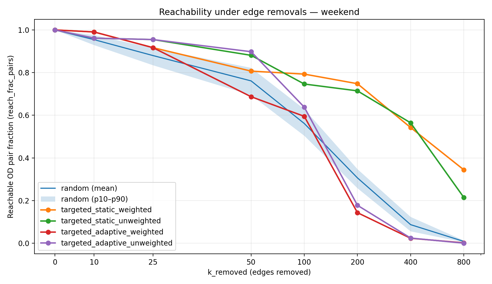
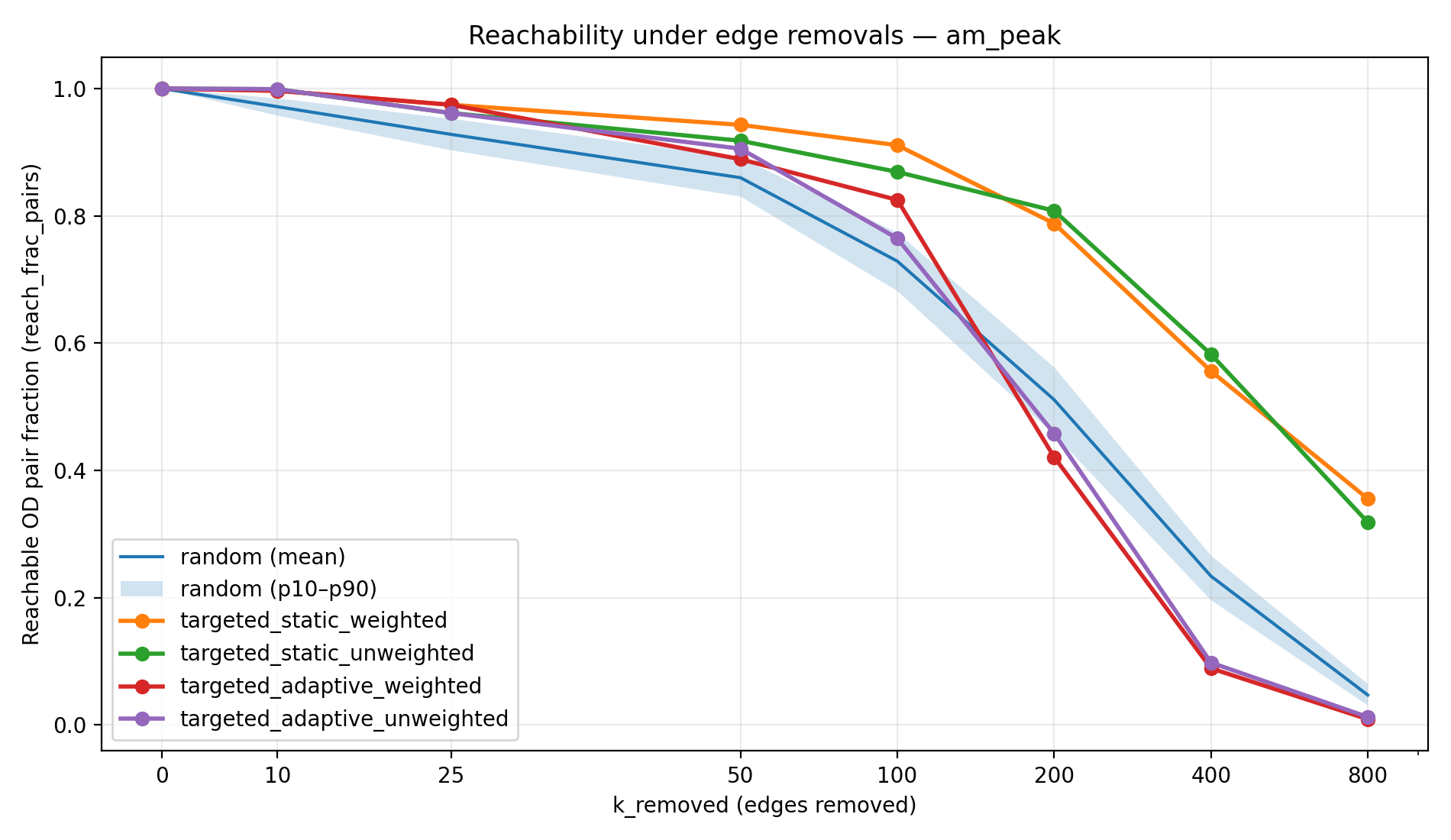
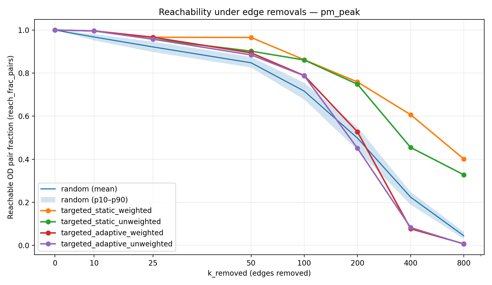
Figure 1a–1d visualizes the reachability trajectories for each scenario. The random strategy is shown as a mean line with a 10th–90th percentile band across 100 Monte Carlo trials, while targeted strategies appear as single curves (deterministic rankings given fixed seeds). This figure is the most direct view of resilience because it shows not only the end state at high k, but also how quickly degradation accelerates, and whether the failure mode is gradual (typical of random damage) versus abrupt (typical of adversarial cascading attacks).
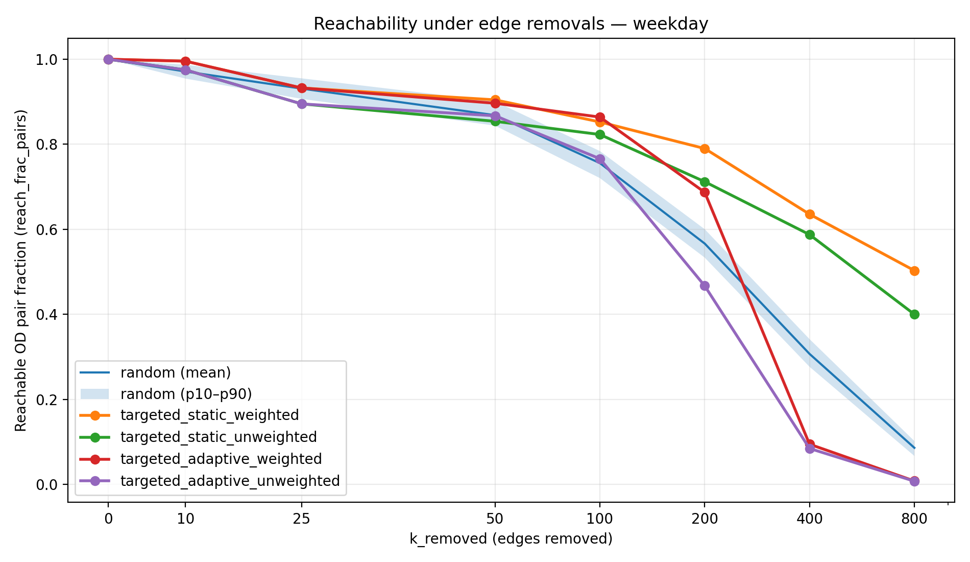
Connectivity Outcomes – Random vs Targeted Removals
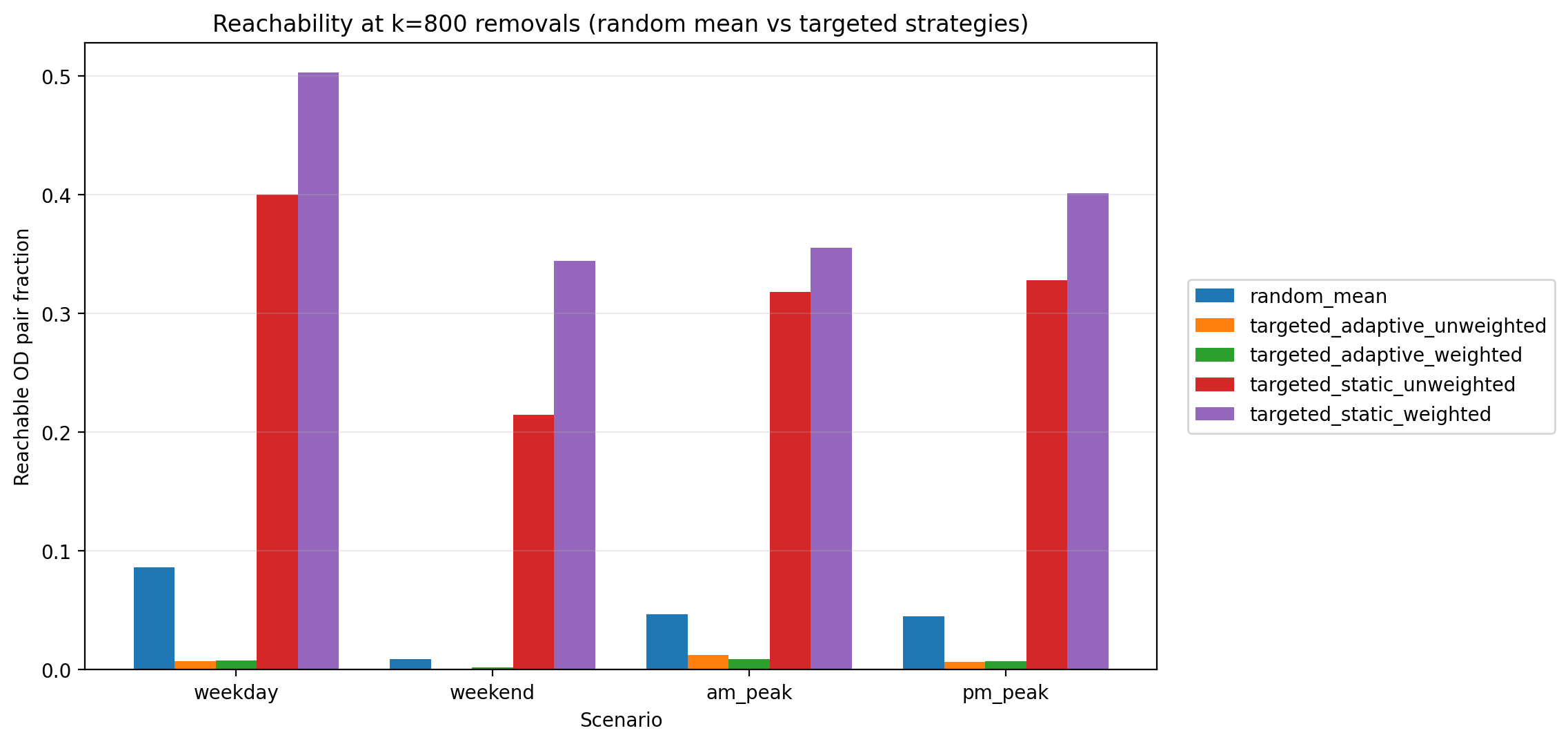
The reachability results show a stark contrast between random failures and targeted attacks. Under random edge removals, the network’s decline is gradual at first—many peripheral or redundant links can be removed with little immediate impact—but eventually reachability falls significantly as critical links are hit. By the extreme of k = 800 random removals, connectivity has collapsed to single-digit percentages of reachable pairs in most cases. For example, in the full weekday scenario only 8.6% of OD pairs remain connected under 800 random failures, meaning over 90% of journeys become impossible. The weekend network is even more fragile, with <1% reachability at 800 random removals. In contrast, the targeted-static strategies (removing the top-ranked corridors from the start) preserve a much larger connected core. Even after 800 targeted-static removals, 20–50% of OD pairs are still reachable (depending on scenario), because alternate routes and redundancies keep large portions of the network connected. Notably, in the weekday scenario the static weighted attack never drove reachability below 50% within the 0–800 removal range. The worst impacts are seen with targeted-adaptive attacks: these approximate a worst-case cascade by continually hitting the next crucial link. Adaptive removals rapidly shatter the network—in all scenarios the reachability at k = 800 is effectively 0% (on the order of 0.1–1% or less). Table 1 summarizes the remaining reachability at the maximum disruption level (800 edges removed) for each strategy and scenario, illustrating how much connectivity each strategy destroys by the end of the simulation.
| Scenario | Random | Static (Wtd) | Static (Unwtd) | Adaptive (Wtd) | Adaptive (Unwtd) |
|---|---|---|---|---|---|
| Weekday | 8.6% | 50.3% | 40.0% | 0.8% | 0.8% |
| Weekend | 0.9% | 34.4% | 21.5% | 0.2% | 0.1% |
| AM Peak | 4.7% | 35.5% | 31.9% | 0.9% | 1.2% |
| PM Peak | 4.5% | 40.2% | 32.8% | 0.8% | 0.7% |
Figure 2 complements Table 1 by showing the same “end state” connectivity comparison at k = 800 as a bar chart. This view makes the ordering visually obvious: static strategies preserve a substantial reachable core, random failures degrade most scenarios to single-digit reachability, and adaptive strategies drive reachability to near-zero across all scenarios. Importantly, Figure 2 also highlights scenario differences—weekend service collapses much more severely under random failures—consistent with a smaller, less redundant network. The end-state fragmentation patterns behind these differences are easiest to see in the maps that follow.
As Table 1 highlights, the static removal strategies maintain a sizeable connected component even under severe attack (e.g., ~50% reachability for weekday static-weighted, vs ~8% under random, at 800 removals). However, this resilience in connectivity comes at the cost of efficiency. Removing the top-weighted corridors forces travelers onto longer detours even though they can still eventually reach their destinations. We observe that path lengths inflate much sooner in the targeted-static scenarios compared to random removal. For example, after 200 edge removals in the weekday scenario, the median travel distance under random failures increased by only ~4% (since most trips could still use near-optimal routes), whereas under static-weighted removals the median trip distance jumped ~27%. In other words, the static strategy immediately knocks out key corridors, so most pairs remain connected but must take longer alternate routes around the gaps.
To make the end-state numbers in Table 1 more tangible, the following maps show what “still connected” looks like after removing 800 edges under different disruption models—and how the network fragments under random versus targeted removal. In particular, Map 2 corresponds to the best-performing connectivity outcome in Table 1 (weekday static weighted ≈ 50% reachability), Maps 3–4 show the near-collapse behavior of random failures at the same disruption level, and Maps 5–6 visualize the weekday network under adaptive attacks (unweighted vs weighted)—the “worst-case” fragmentation patterns consistent with the near-zero reachability in Table 1.
Maps 5-6 make the “adaptive” result in Table 1 concrete: once the attack recomputes importance after each disruption, it repeatedly removes the new bottleneck created by earlier removals. Visually, this turns what remains of the weekday core (already thinned under random failures in Map 4) into scattered fragments—exactly the kind of cascade-like breakdown that drives reachability toward ~0% by k = 800.
Figure 3a–3d makes this “connectivity vs efficiency” distinction explicit by plotting the penalized path length ratio versus k (on a log scale). The penalized metric is computed by assigning newly unreachable OD pairs a large penalty distance, which keeps the average comparable as the graph fragments. Without this penalty, average travel distance among the remaining reachable pairs can become misleading at high k (because unreachable trips drop out of the average). The log scaling is useful because the metric grows slowly early on and then accelerates rapidly once disconnections become widespread.
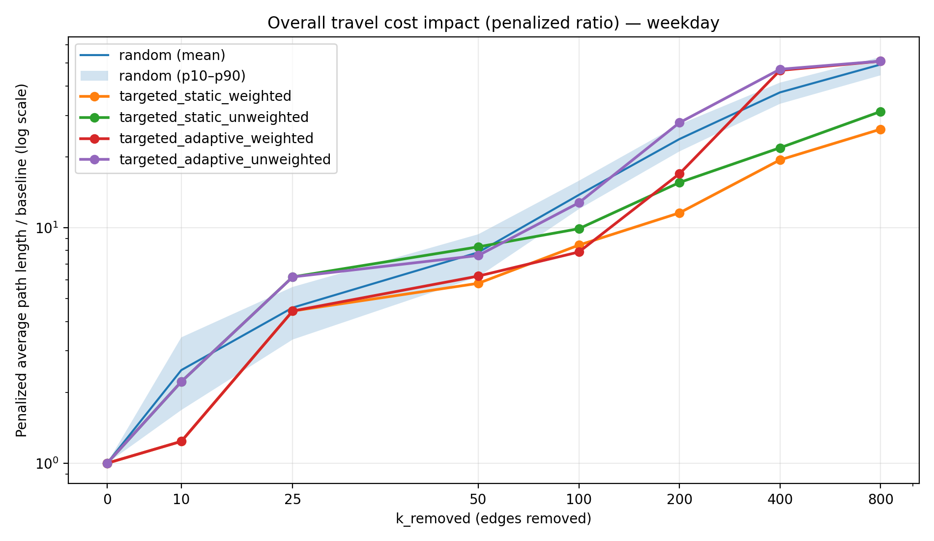
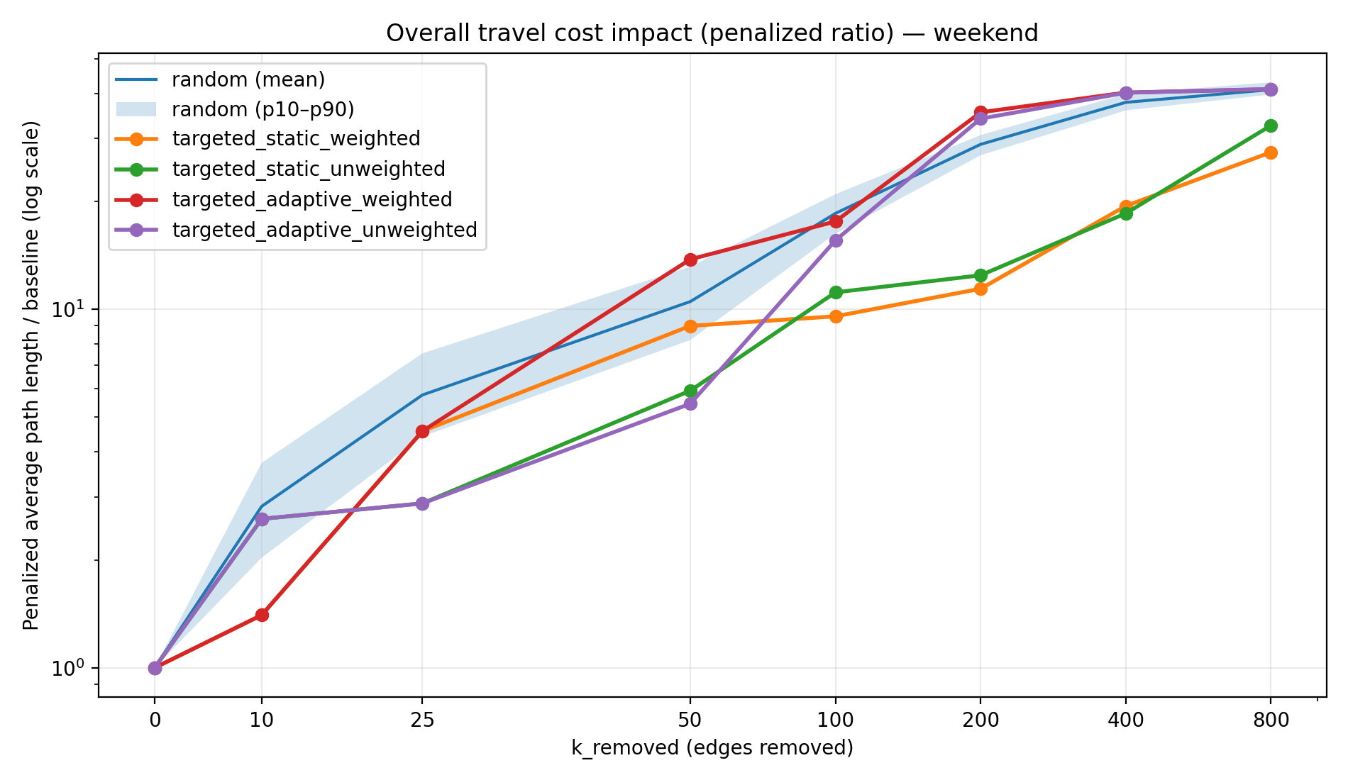
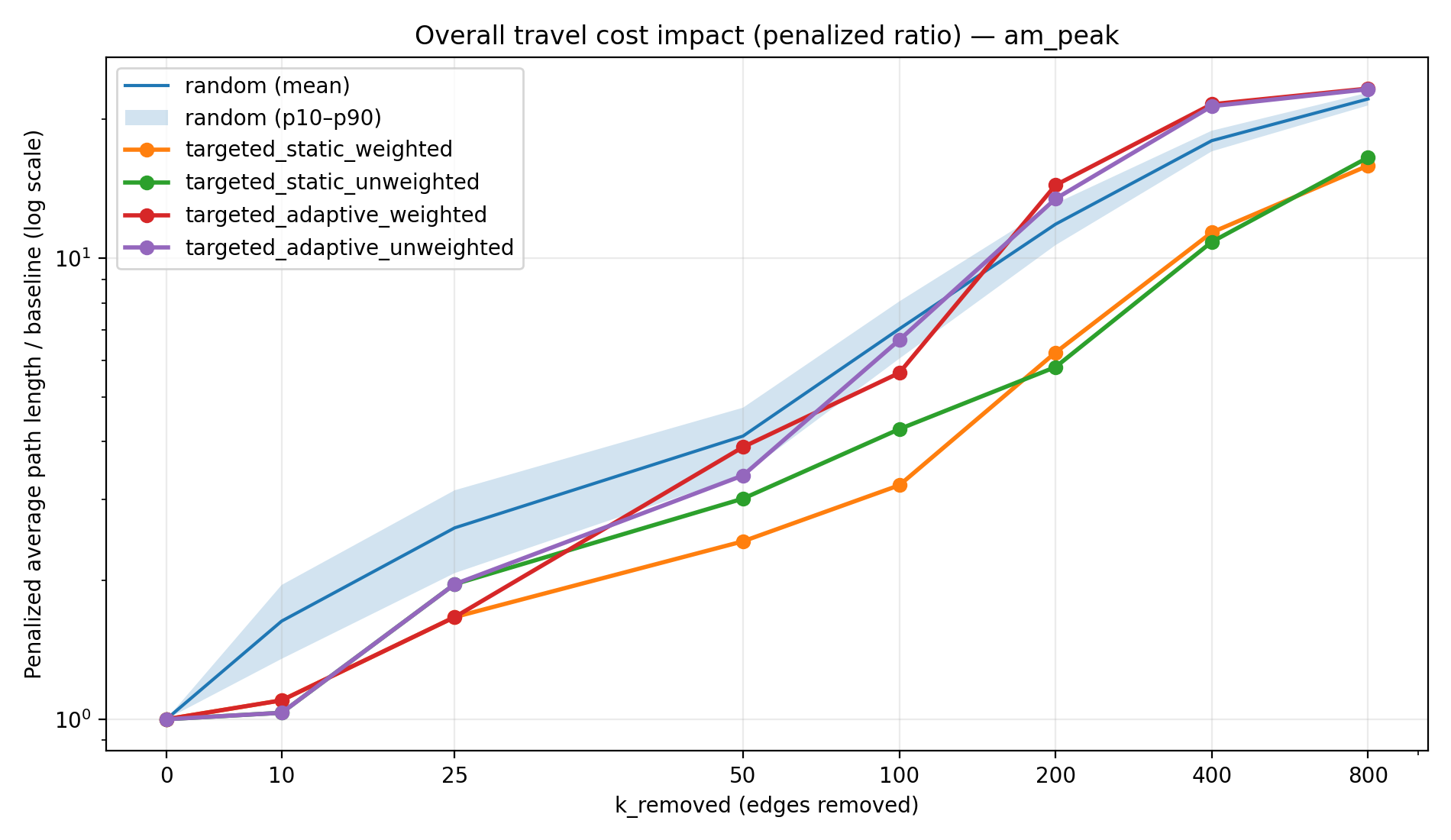
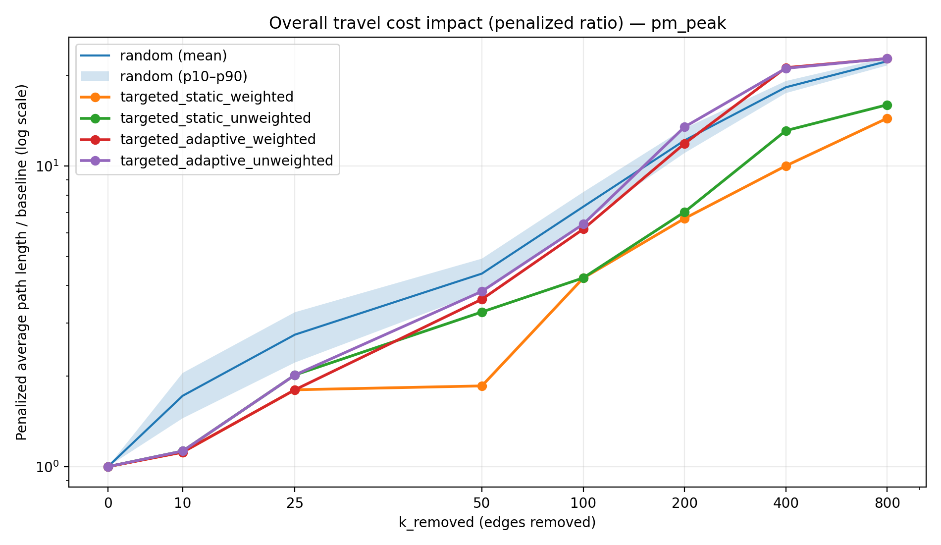
By the time we reach 800 removals, the penalized path length ratio (average effective trip length relative to baseline) is dramatically higher for random and adaptive strategies due to massive disconnections, while static strategies—though still causing detours—have lower overall penalty. Table 2 shows the penalized path length ratio at k = 800. For instance, on a weekday the random failures yield an average effective travel distance ~49.5× the baseline (virtually every trip is either extremely long or unattainable), whereas the static-weighted strategy yields about 26× baseline—a substantial increase, but roughly half the penalty of random removal. The adaptive attacks are again the most severe, with path length ratios on par with or worse than random (approaching 50× baseline in the worst cases). Notably, the static strategies keep this metric far lower by preserving connectivity in a large portion of the network—travel distances increase due to rerouting, but at least those trips still exist. In contrast, random and adaptive removals leave so many pairs disconnected that the penalized average soars.
| Scenario | Random | Static (Wtd) | Static (Unwtd) | Adaptive (Wtd) | Adaptive (Unwtd) |
|---|---|---|---|---|---|
| Weekday | 49.5× | 26.2× | 31.2× | 51.0× | 51.0× |
| Weekend | 41.0× | 27.4× | 32.6× | 41.1× | 41.2× |
| AM Peak | 22.2× | 15.9× | 16.5× | 23.3× | 23.3× |
| PM Peak | 22.3× | 14.4× | 16.0× | 22.7× | 22.8× |
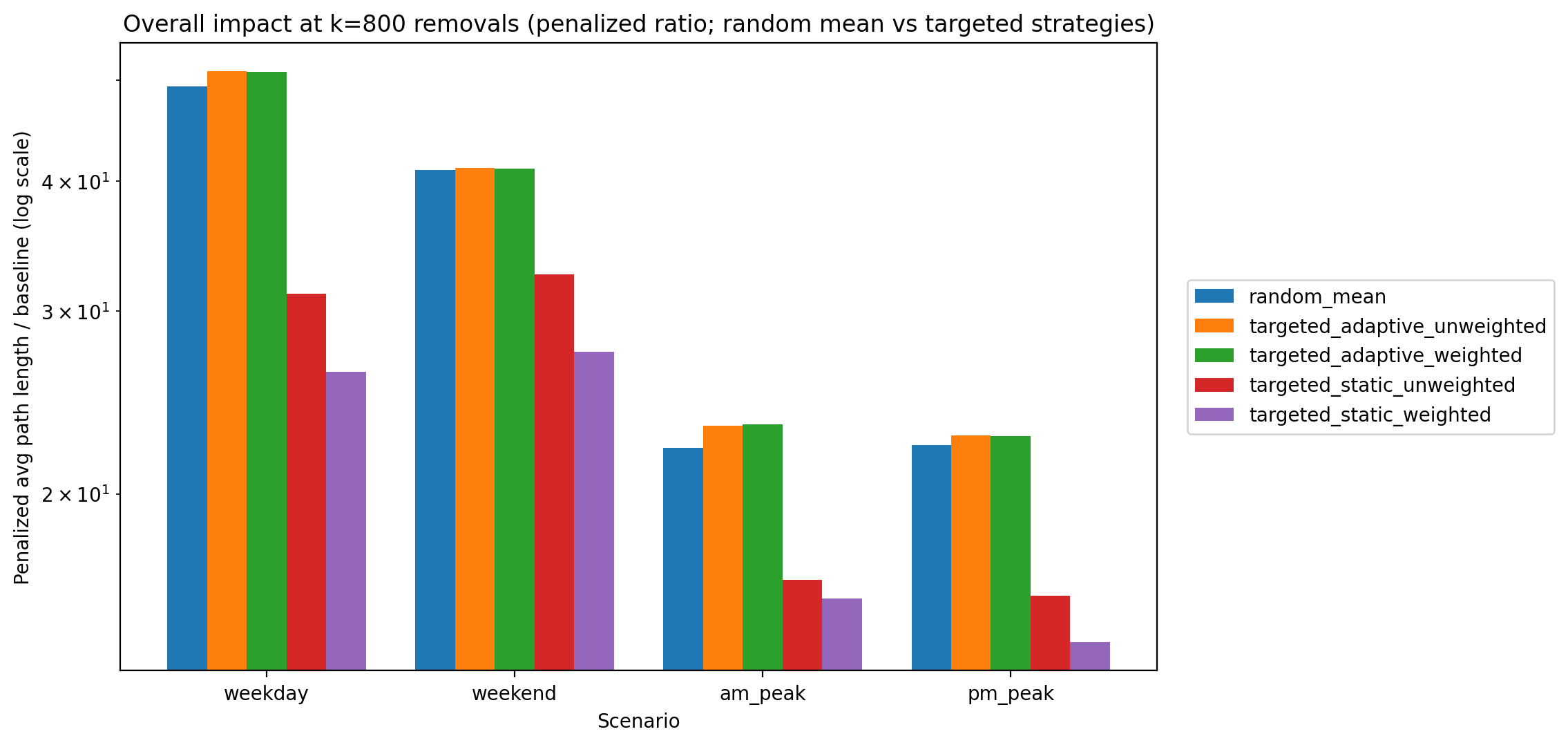
Figure 4 summarizes Table 2 in a single comparative view at k = 800. This figure is helpful because it shows that “disconnecting the city” and “making travel painfully inefficient” are related but not identical outcomes. Static strategies frequently preserve OD reachability, but still incur meaningful detour costs, while random and adaptive strategies impose extreme penalties because a large fraction of OD pairs becomes unreachable. In practical terms, static corridor removals resemble “the network still works but trips become much longer,” whereas random and adaptive removals resemble “large portions of the city become unreachable.”
These findings illustrate a clear connectivity–efficiency trade-off in the network’s resilience. The static targeted removals cause efficiency degradation long before the network suffers connectivity collapse. In those scenarios, the largest weakly connected component still contains most of the nodes (as measured by LWCC size; e.g., ~80–90% of nodes remain in one giant component for static strategies at k=800), meaning the network is physically still intact; yet many trips become much longer because direct routes are disabled. On the other hand, the random and adaptive strategies lead to rapid connectivity collapse—large portions of the network become completely isolated, which is reflected in the very low reachability and extreme path length ratios for those cases. It’s worth noting that by the end of the process (800 removals), random failures and adaptive attacks inflict a similar level of total damage (both effectively sever most of the network, as seen in Tables 1 and 2). The crucial difference is how quickly that damage accumulates. A random failure sequence might require hundreds of removals to knock out half the trips, whereas an intelligently targeted (adaptive) sequence often achieves the same level of disruption with fewer removals (Table 3).
Table 3 underlines this difference by listing the approximate number of edge removals (k level) required for reachability to drop below 50% in each scenario. The targeted-adaptive strategies are the most aggressive: in most cases, ~200–400 targeted removals are enough to break the network’s connectivity in half (and beyond that point, reachability free-falls toward zero). For example, in the weekday scenario, the adaptive-unweighted attack drove reachability below 50% after only ~200 removals, and by 400 removals it had wiped out over 90% of connectivity. The random failure scenarios typically needed roughly 200–400 removals to cross the 50% reachability threshold (e.g., around ~400 for weekday and ~200 for the smaller weekend network). Meanwhile, the targeted-static strategies were far more resilient by this measure: in several cases reachability never fell below 50% even at 800 removals (denoted “>800” in the table). For instance, weekday static-weighted removal still retained slightly above 50% reach at k=800, implying that more than 800 strategic failures would be required to split the network’s connectivity in half. Even in scenarios where static removals eventually did drop below half reachability (such as weekend static-unweighted), the threshold wasn’t reached until very late in the attack (around 800 removals). This ordering—static (best), random (middle), adaptive (typically worst, with scenario-specific exceptions)—demonstrates how network redundancy and the manner of disruption determine the speed of collapse.
| Scenario | Random | Static (Wtd) | Static (Unwtd) | Adaptive (Wtd) | Adaptive (Unwtd) |
|---|---|---|---|---|---|
| Weekday | ~400 | >800 | 800 | ~400 | ~200 |
| Weekend | ~200 | 800 | 800 | ~200 | ~200 |
| AM Peak | ~400 | 800 | 800 | ~200 | ~200 |
| PM Peak | ~200 | 800 | ~400 | ~400 | ~200 |
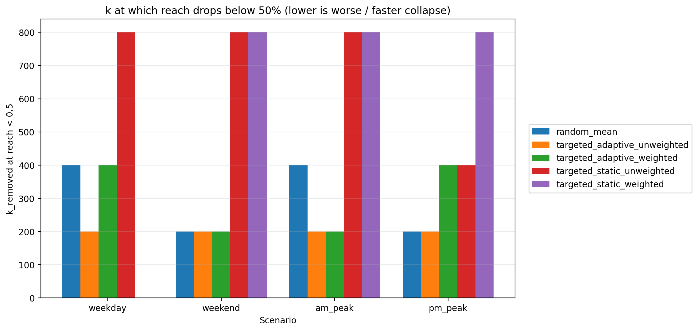
Figure 5 visualizes Table 3 as a “time-to-failure” plot, where lower bars indicate a faster collapse (fewer removals needed to push reachability below 50%). This is a useful graphic because it converts the full reachability trajectories into a single, interpretable number. It also makes the hierarchy of resilience visually clear: adaptive strategies typically fail fastest (though some scenarios are comparable to random), random failures are intermediate, and static strategies are slowest to cross the 50% threshold (or do not cross it within k≤800).
Scenario Fragility and Network Redundancy
The resilience patterns above are strongly influenced by each scenario’s network structure. The weekday network (full weekday service) is the most robust: it has the highest route density and overlapping corridors, providing alternative paths when some links fail. This is evident in the results—for instance, the weekday scenario maintains the largest reachability across all strategies (Table 1) and requires more removals to cripple (Table 3) compared to the same strategies in other scenarios. In practical terms, a weekday transit network has many parallel routes and more frequent service, so even if a major corridor is removed, riders can often backtrack or use a different line to reach their destination (albeit with a delay). The weekend network, by contrast, is much more fragile. With fewer routes in operation and lower frequency, the weekend scenario lacks redundancy: many areas are connected by only a single line or a sparse set of transfers. As a result, removing even a moderate number of edges can isolate large portions of the network. We saw that under random failures, the weekend reachability dropped below 50% after roughly half the number of removals needed on a weekday (~150 vs ~300), and ultimately plummeted to under 1% at k=800 (Table 1). Even targeted-static removals, which perform best, left only 21–34% reachability in the weekend case (versus ~40–50% on weekday). This underscores that lower network redundancy and corridor density in the weekend scenario make it inherently less resilient to disruptions.
The peak-hour scenarios (AM Peak and PM Peak) show intermediate resilience. During peak times, transit networks often add express or additional routes, but these tend to concentrate on key corridors. Our results indicate that the peak scenarios behave similarly to the weekday network but with slightly lower robustness. For example, by 800 removals the PM Peak network under static-weighted attack retained ~40% reach (versus 50% on the full weekday network), and the threshold for 50% connectivity was around 400 removals for one of the peak static cases (Table 3) whereas the weekday needed more. This suggests that while peak networks have more routes than the weekend (improving redundancy), they may rely heavily on a few critical arteries (e.g., main downtown feeders)—making them somewhat more vulnerable than the broader all-day network. In general, adding routes (as in weekday service) distributes the load and creates fallback options, whereas route cuts (as in weekend service) concentrate travel onto single points of failure.
Adaptive Cascades vs. Static Attacks
Finally, it is important to emphasize why the adaptive strategies are especially devastating—they effectively simulate a cascading failure or intelligent adversary scenario. In a static attack, the list of target edges is determined upfront (e.g., the highest-frequency corridors from the original network). Once those top targets are removed, the network might reconfigure—some remaining links become more critical as traffic reroutes, but the static strategy doesn’t account for that. In contrast, an adaptive removal continually finds the new weakest link after each failure. This means early removals weaken the network, and subsequent removals strike at the newly exposed critical links, causing compounding damage. The outcome is a worst-case trajectory: connectivity disintegrates far faster than under any static or random process. In our simulation, the adaptive methods aggressively fragmented the network—for instance, after ~200 adaptive removals in several scenarios (and by ~400 in the remaining cases), reachability dropped below half (Table 3). By 400 removals, most adaptive runs had effectively obliterated the network’s connectivity (e.g., <10% reach remained). These adaptive results mimic scenarios like an escalating cascade (where one failure overloads other parts of the system, leading to more failures) or a strategic attack on infrastructure. They demonstrate the transit network’s worst-case vulnerability: even though the network has built-in redundancy, a coordinated series of hits on major transfer points and corridors can rapidly dismantle its integrity.
In summary, our results paint a two-fold picture of resilience. On one hand, the transit network exhibits robustness to random failures—it can tolerate many minor disruptions before connectivity truly collapses, thanks to redundant paths and a large interconnected core (especially on weekdays). On the other hand, the network is highly vulnerable to targeted, compounding disruptions that exploit its weaknesses. The connectivity collapse under worst-case removals is abrupt and severe, whereas under more benign scenarios the network mostly experiences a gradual efficiency degradation (longer routes but still connected). These findings reflect the underlying network structure: a dense web of routes that can handle isolated outages, but with certain critical corridors whose loss can cascade into system-wide breakdowns. The differences across scenarios highlight how service levels and network design (route density on weekdays vs. weekends, etc.) influence resilience. Overall, the study underscores the importance of identifying key corridors and nodes that serve as load-bearing elements in the network—bolstering those or providing alternatives could significantly improve resilience against worst-case failures.
Discussion
This project set out to measure how a GTFS-derived transit network degrades under progressive disruption, and the results support a clear hierarchy of resilience outcomes: static targeted removals preserve a connected core the longest, random failures erode connectivity more gradually but ultimately collapse, and adaptive targeted removals behave like worst-case cascades that rapidly fragment the network. The most important takeaway is that “resilience” is not a single property. The network can remain largely connected while becoming substantially less usable (efficiency degradation), or it can remain locally efficient for many trips until it suddenly becomes unusable for large parts of the city (connectivity collapse). The different strategies emphasize these distinct failure modes.
Random failures are not benign, but they fail slowly
Random removals produce the most intuitive curve shape: early removals often hit peripheral or redundant links, so reachability declines slowly at first. But the eventual collapse at high k shows that even “ordinary” disruption can severely damage the system once it begins striking corridors that happen to be structurally important. The wide 10th–90th percentile band in random trials also matters: resilience under random failures is not a single story but a distribution of possible outcomes. Some random sequences “get lucky” and avoid critical corridors longer; others hit them early. That variance is itself a practical insight: even without an adversary, a transit system can experience very different disruption severities depending on which specific links fail.
Static targeted removals reveal a connectivity–efficiency trade-off
Static targeted removals were the most resilient in reachability, particularly in the weekday scenario, where a sizeable OD-connected core survived even at high removals. But the penalized path length ratios show why this should not be interpreted as “the network is fine.” Static strategies immediately remove high-importance corridors, so many OD pairs remain connected only by detouring through less direct paths. In other words, static targeted removals preserve existence of paths while degrading quality of paths early.
This trade-off has an intuitive operational interpretation. A network with many alternative pathways can route around lost corridors, but those reroutes can be costly: longer travel times, more transfers, and less predictable service. In planning terms, the static curves imply that systems can remain “connected on paper” while riders experience substantial usability loss well before total disconnection becomes obvious.
Adaptive targeted removals approximate cascading failure
Adaptive strategies stand out as the most destructive because they actively exploit the network’s evolving vulnerability. When the most critical edge is removed, traffic (in a shortest-path sense) reroutes and concentrates on new bottlenecks. Recomputing betweenness after each removal repeatedly strikes these newly exposed choke points. That mechanism explains the steep decline in reachability and the near-zero connectivity by k = 800 across scenarios: the strategy is not merely removing “important” edges, it is removing the next edge that becomes important as the system reacts.
Substantively, this is the closest analog in the study to a cascading failure process. It mirrors real-world dynamics where disruptions can compound: a closure forces rerouting, rerouting overloads transfer points or parallel corridors, and those weak points become more likely to fail or become unusable. While the project does not model capacity directly, the adaptive results still provide a rigorous upper bound on how quickly the network can fragment under compounding, strategically aligned failures.
Scenario differences are structural, not cosmetic
The scenario ordering is consistent with a redundancy explanation:
- Weekday service is the most resilient because it contains the densest set of overlapping corridors and transfer opportunities. Even targeted disruptions leave enough alternate paths to preserve a large connected core.
- Weekend service is the most fragile, especially under random failures, because reduced service tends to eliminate parallel paths. When redundancy is low, many links act as bridges: losing a small set of them isolates whole regions.
- Peak networks sit in between: they can be well-connected in core commute corridors, but they may depend heavily on a concentrated set of downtown feeders and transfer links.
The weekend results are particularly important: they suggest that reduced service is not just “fewer trips,” but a different network topology—one that is structurally more vulnerable to both random and targeted disruptions. This has a practical implication: resilience planning cannot assume that weekday robustness generalizes to weekends. A corridor that is redundant on weekdays may become a single point of failure on weekends.
What “weighted vs. unweighted” means in practice
The weighted and unweighted strategies target different notions of criticality. Unweighted centrality tends to highlight structural bridges and high-flow topological connectors—edges that sit on many shortest paths regardless of service intensity. Weighted centrality shifts focus toward edges that reduce generalized travel cost, which in transit tends to reward frequent, fast, or otherwise high-utility corridors. The results show that these two perspectives can produce meaningfully different disruption outcomes depending on scenario:
- Weighted targeting can remove the “best” corridors early, often preserving connectivity through worse corridors (large efficiency hit, slower connectivity collapse).
- Unweighted targeting can sever structural bridges, accelerating fragmentation even if the removed links are not the highest-frequency corridors.
This distinction is valuable for interpretation. If the goal is rider-centered robustness, weighted criticality aligns with “high-value” segments. If the goal is pure connectivity resilience, unweighted criticality aligns with structural weak points. The divergence between these approaches helps explain why a network can appear operationally strong (high-frequency corridors) while still being structurally brittle (bridge-like links).
Why the results can look counterintuitive at first glance
One potentially surprising outcome is that static targeted attacks can preserve reachability better than random failures at high k. This is not a contradiction; it reflects the difference between how connectivity is lost versus how efficiency is lost. Static attacks remove major corridors, but they do not adapt to the shifting bottlenecks. The network “finds a way” to keep many OD pairs connected, but via increasingly inefficient routes. Random attacks, by contrast, eventually hit enough structural bridges—by chance—that the giant component collapses, even if efficiency for remaining reachable pairs was relatively stable earlier. Adaptive attacks combine the worst of both worlds: they deliberately create fragmentation and then exploit the fragmentation process.
Limitations
Several limitations are worth stating explicitly to keep the findings properly scoped:
- GTFS-only travel costs are a proxy. The generalized weight captures schedule-based structure (time and frequency), not real-time delays, capacity, reliability, crowding, or transfer penalties beyond what is implied by frequency.
- Demand is not modeled. OD pairs are sampled from reachable baseline pairs rather than weighted by observed ridership or land use. The results describe structural resilience, not ridership-weighted equity or welfare impacts.
- Edge removal is an abstraction. Removing a stop-to-stop edge corresponds to a disrupted segment in the schedule graph, not necessarily a physical road closure. Some real disruptions would remove multiple edges or entire routes simultaneously; others might reduce frequency rather than remove connectivity outright.
- Adaptive attacks are intentionally adversarial. They are best interpreted as an upper bound / worst-case stress test, not a prediction of typical disruption sequences.
- Map rendering can understate “removed segments.” When edges are drawn along GTFS shapes, a directed edge may map to only a segment of a longer shape polyline. Visual gaps can therefore reflect routing choices in the shape-matching procedure rather than a failure of the underlying graph logic.
These limitations do not invalidate the results; they clarify what the results are: a structural analysis of schedule-derived connectivity under stylized disruption processes.
Implications for resilience planning and service design
Even with these limits, the findings support several actionable interpretations:
- Redundancy matters more than raw size. Weekday resilience appears tied to overlapping corridors and multiple transfer options. Weekend fragility suggests that service cuts can create bridge-like links and choke points that dominate connectivity.
- Protecting critical edges depends on the failure model. If the concern is everyday random disruption, improving robustness may mean adding redundancy broadly (more alternate paths). If the concern is worst-case cascading failure, it may mean strengthening or backing up structural bridges and transfer bottlenecks identified by adaptive or unweighted centrality.
- Connectivity preservation is not enough. Static strategies show that a network can remain connected while travel becomes far more circuitous. Resilience planning should therefore track both reachability and efficiency (or user cost), not only component size.
- Scenario-aware planning is essential. Weekend and peak networks should be evaluated separately, because their topology and redundancy differ meaningfully from the full weekday network.
Next steps
The most natural extensions (still consistent with a GTFS-only constraint) would be:
- Node-centric criticality: identify stops whose removal (or incident) fragments the network most severely, complementing edge-centric analysis.
- Equity-aware OD sampling: stratify OD pairs by geography (e.g., zone-based sampling) to see whether disconnections disproportionately isolate certain areas.
- Frequency degradation instead of edge deletion: simulate service cuts by reducing edge frequency (increasing expected waiting) rather than removing edges entirely, which may better match many real-world disruptions.
- More interpretable “critical corridor” summaries: cluster high-criticality edges into corridor-level groups to produce narrative outputs like “top 10 load-bearing corridors” per scenario.
Overall, the results support a coherent story: the transit network is moderately robust to random damage, fragile under compounding targeted disruptions, and highly sensitive to service pattern–driven redundancy. Static targeted disruptions expose a hidden vulnerability: the network may stay connected while becoming operationally inefficient. Adaptive disruptions expose the worst-case vulnerability: connectivity can collapse rapidly when failures align with evolving bottlenecks. This duality—connectivity vs. efficiency, random vs. targeted, weekday vs. weekend—captures the central resilience lesson of the study.
Conclusion
This project used a GTFS-only representation of the Metro Transit network to quantify criticality and resilience across four operating scenarios (weekday, weekend, AM peak, PM peak) under progressive edge removals. By combining schedule-derived connectivity with repeated disruption simulations, the analysis demonstrates that the network’s robustness depends as much on how failures occur as on how many links are lost.
Three conclusions stand out.
First, random failures degrade the system gradually but still lead to severe collapse at high disruption levels. Many early removals have limited impact because they strike redundant or peripheral links, but continued losses eventually fragment the network and drive reachability toward very low levels—especially in structurally smaller service patterns such as weekends.
Second, static targeted removals preserve connectivity better than random failures but impose large efficiency costs early. Removing a predetermined set of “most important” edges can leave a sizable connected core intact even under heavy disruption, yet the network becomes substantially less usable because remaining trips require long detours. This reveals a key resilience trade-off: a network may remain connected in a graph-theoretic sense while becoming practically inefficient for riders.
Third, adaptive targeted removals approximate worst-case cascades and are consistently the most damaging. By recalculating importance after each failure, the adaptive strategy repeatedly removes the next bottleneck created by prior removals, rapidly accelerating fragmentation and driving reachability to near zero across scenarios. These results provide a plausible upper bound on vulnerability under compounding disruptions and highlight how quickly the network can unravel when failures align with evolving choke points.
Across scenarios, the study shows that redundancy is the dominant driver of resilience. Weekday service—denser and more overlapping—sustains connectivity longer than weekend service, which is inherently more fragile because it contains fewer alternative paths and more bridge-like dependencies. Peak service falls between these extremes, retaining some redundancy but also concentrating connectivity into core commuter corridors.
Overall, the analysis supports a clear operational interpretation: transit networks can be robust to isolated disruptions but remain vulnerable to coordinated or compounding failures, and maintaining “connectivity” alone is not sufficient for rider-relevant resilience. Identifying and reinforcing load-bearing corridors and transfer structures—while also preserving alternate routing options, especially in reduced-service scenarios—appears central to improving resilience.
Future work can extend this GTFS-only framework by simulating frequency reductions rather than hard removals, evaluating node failures (stop-level disruptions), and incorporating equity-aware OD sampling to understand which neighborhoods become isolated first. Even in its current form, the project provides a reproducible methodology for ranking critical links, stress-testing service patterns, and communicating resilience outcomes with interpretable metrics and maps.