Introduction

Breast cancer remains a significant global health challenge, necessitating reliable and efficient diagnostic tools for timely intervention and improved patient outcomes. In this analysis, we present an analysis of breast cancer diagnosis using the Breast Cancer Wisconsin (Diagnostic) dataset. To predict breast cancer diagnoses, we employ logistic regression, a statistical method widely used for binary classification tasks. After performing feature selection, we implement Principal Component Analysis (PCA), a dimensionality reduction technique that transforms the high-dimensional dataset into uncorrelated principal components. This preprocessing step ensures the model’s robustness and accuracy in predicting breast cancer diagnoses based on the selected and transformed features. This analysis gives insight into the application of logistic regression and PCA in breast cancer diagnosis. The findings hold significant potential for supporting early detection and intervention efforts in breast cancer diagnosis, ultimately contributing to improved patient care and outcomes.

Data

In this analysis, we utilize the Breast Cancer Wisconsin (Diagnostic) dataset. This data was collected and made available by researchers at the University of Wisconsin, Madison, and the University of California, Irvine.

The data was originally obtained for the purpose of breast cancer research and diagnosis. It includes features extracted from digitized images of fine needle aspirates (FNA) of breast masses, which were collected from patients with suspected breast cancer. Fine needle aspiration is a minimally invasive procedure where a thin needle is used to extract cells from a breast mass or lump for examination.

The dataset consists of 569 instances, with each instance representing a breast mass. For each mass, the following features were computed from the digitized images:

• Ten real-valued features computed for each cell nucleus present in the image:
  • Radius (mean of distances from the center to points on the perimeter).
  • Texture (standard deviation of gray-scale values).
  • Perimeter.
  • Area.
  • Smoothness (local variation in radius lengths).
  • Compactness ($\frac{\text{perimeter}^2}{\text{area} - 1.0}$).
  • Concavity (severity of concave portions of the contour).
  • Concave points (number of concave portions of the contour).
  • Symmetry.
  • Fractal dimension (“coastline approximation” - 1).
• The mean, standard error, and “worst” (mean of the three largest values) of these ten features were also computed, resulting in a total of 30 features.
• The diagnosis label for each instance, which is either “M” (Malignant) or “B” (Benign).

Methods

In our study, we are conducting a logistic regression analysis on the Breast Cancer Wisconsin (Diagnostic) dataset to predict the likelihood of breast cancer diagnoses. Logistic regression is a statistical method used for binary classification tasks, where the goal is to predict the probability that an instance belongs to one of two possible classes. It is a type of regression analysis that models the relationship between the input features (independent variables) and the probability of a specific outcome (dependent variable) using the logistic function. The logistic function (sigmoid) maps the predicted values to a range between 0 and 1, representing the probability of the positive class. The model estimates the coefficients of the input features, allowing us to make predictions and understand the impact of each feature on the outcome.

However, before applying logistic regression, we recognize that the dataset suffers from multicollinearity issues, where some of the features are highly correlated, potentially leading to unstable regression coefficients and unreliable predictions. To mitigate this problem, we first perform feature selection using our domain knowledge to identify and eliminate several features. This step helps us retain the most discriminative variables while reducing the risk of multicollinearity.

After feature selection, we employ Principal Component Analysis (PCA) to further transform the data into uncorrelated principal components. Principal Component Analysis (PCA) is a dimensionality reduction technique used to transform a high-dimensional dataset into a lower-dimensional space while retaining the most significant patterns or variations in the data. It does this by identifying the principal components, which are new uncorrelated variables that are linear combinations of the original features.

By extracting the principal components, we can create a new set of orthogonal variables that capture the maximum variance in the data while minimizing the correlation between them. This preprocessing step ensures that our logistic regression model will be more robust and accurate in predicting breast cancer diagnoses based on the selected and transformed features, ultimately enhancing the overall quality of our analysis.

Results

To enhance our feature selection process, we focus on eliminating certain variables to address multicollinearity effectively. The “error” variables in the dataset are suitable candidates for elimination because they represent the standard error of the corresponding “mean” variables. Eliminating these “error” variables reduces multicollinearity because the “error” variables are derived from and closely related to the “mean” variables.

We may also eliminate two of the “radius”, “area”, and “perimeter” variables. All three are also closely related, as they are inherently related geometrically. We will eliminate all but the “radius” variables to mitigate the problem of multicollinearity. We have kept the “radius” variables rather than “area” or “perimeter” due to clinical utility. Radius estimates are often the most utilized value in imaging reports. By carefully selecting and eliminating features based on their correlations and clinical relevance, we aim to enhance the reliability and interpretability of our logistic regression analysis.

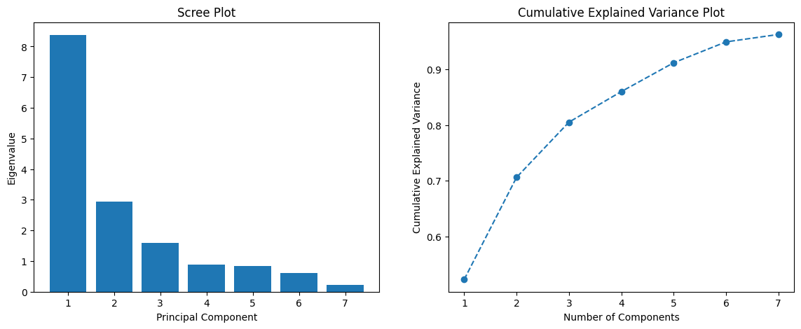
We summarize the results of our principal component analysis in figures 1 and 2. The left graph shown in figure 1 shows the eigenvalues (variance explained) by each principal component. The rapid decline indicates that the first few components capture a significant amount of the variance, while the latter components add progressively less information. On the right, one can observe how the cumulative variance explained increases as we consider more components. It is evident that around 7 components explain roughly 95% of the variance, consistent with the previous result.

Figure 1 (Scree Plot and Cumulative Explained Variance):

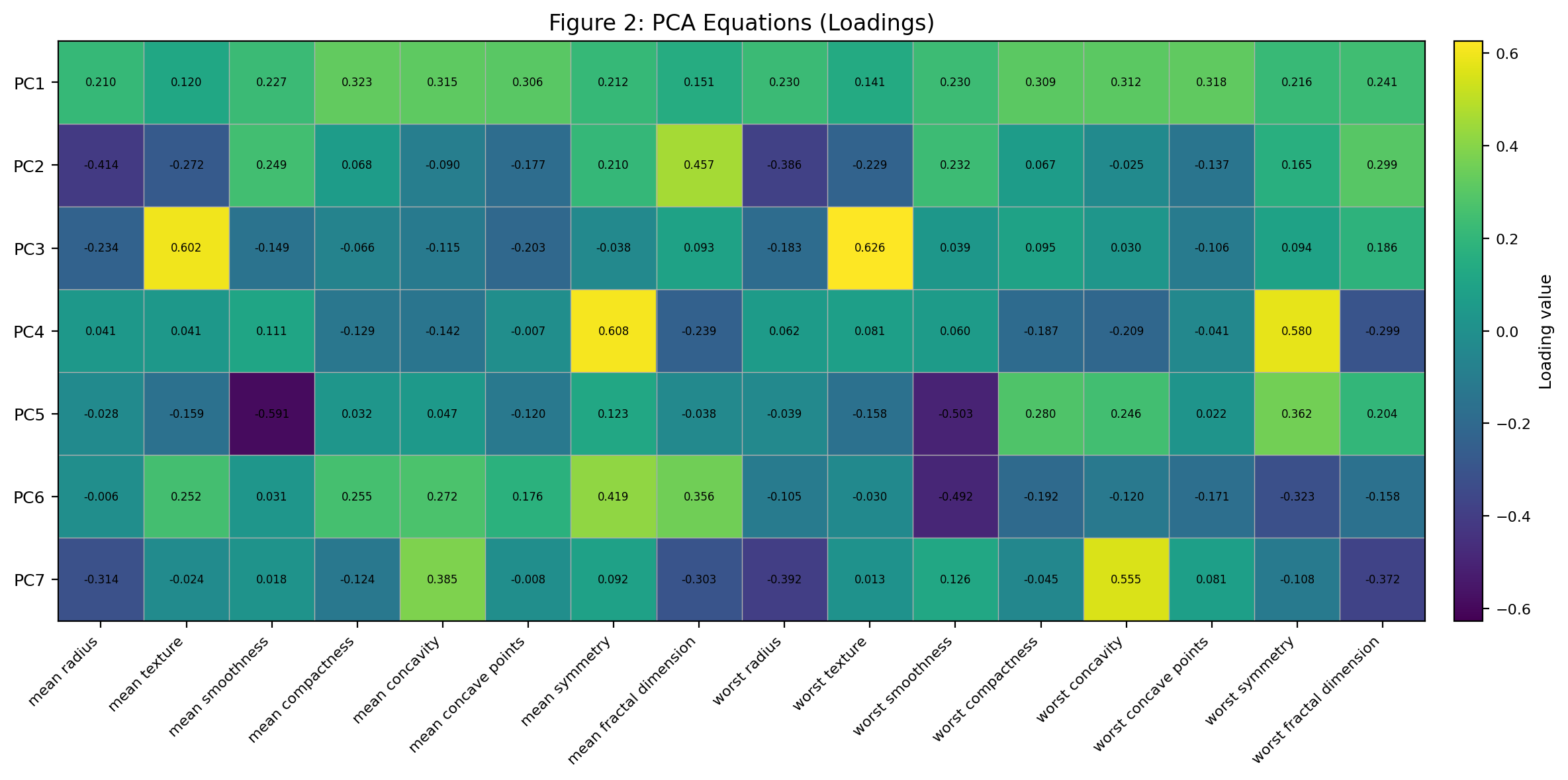
The equations of each principal component are shown in figure 2. In figure 2, each row in the table corresponds to a principal component (PC), and each column corresponds to an original feature from the dataset. The values indicate the weight or loading of each feature in the respective principal component. For instance, for PC_1: “mean radius” has a loading of 0.210402; “mean texture” has a loading of 0.119592, and so on. These loadings can be interpreted as the correlations between the original features and the principal component. A high absolute value for a loading indicates that the respective feature has a strong influence on that principal component. Positive and negative values indicate the direction of the correlation with the principal component. By examining the loadings for each PC, we get an idea of which original features are most influential for each component. This can help in interpreting the “meaning” or “character” of each PC in terms of the original features. For example, if we look at PC1, it seems to give significant weight to features like “mean compactness”, “mean concavity”, “mean concave points”, and so on. This suggests that PC1 might represent some aspect of the overall compactness or shape of the tumor cells.

Figure 2 (PCA Equations):

We now summarize the results from the logistic regression on the PCA-transformed data:

• Accuracy: 97.2%
• Classification Report
  • For Class 0 (Malignant)
    • Precision: 95%
    • Recall: 98%
    • F1-score: 96%
  • For Class 1 (Benign)
    • Precision: 99%
    • Recall: 97%
    • F1-score: 98%

The full model is

Where:

And PC_i is listed in Figure 2.

Interpreting the coefficients in terms of odds ratios is straightforward. A one-unit increase in PC_i is associated with a change in the odds of the tumor being benign by a factor of e^β, where β corresponds to the coefficient of PC_i in the logistic regression (-2.0553, 2.0482, etc.).

Perhaps visualization is more interesting than the interpretation of our model. Figure 3 provides a special representation of the data when projected onto the first two principal components. Each point in this plot represents a tumor sample. The x-axis corresponds to the first principal component (PC1), and the y-axis corresponds to the second principal component (PC2). The colors (red for malignant and blue for benign) represent the true labels of the samples. From this plot, we can observe that there’s a general separation between the two classes, suggesting that the first two PCs capture some of the variance that differentiates between benign and malignant tumors. However, there’s still some overlap, indicating that the distinction isn’t perfect in this 2D space.

Figure 3 (2D Scatter Plot of the first two Principal Components with True Labels):

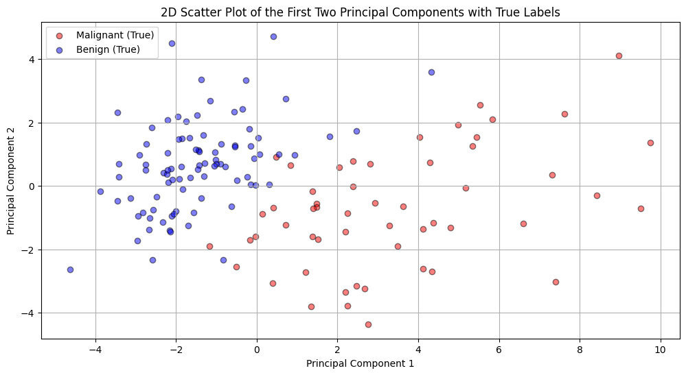
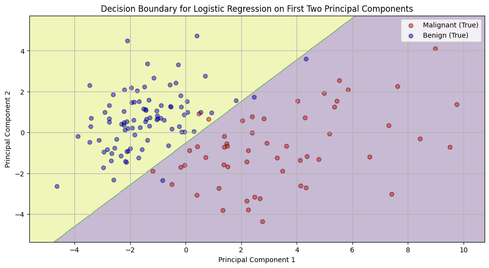
Figure 4 visualizes how the logistic regression model classifies data points in the space of the first two PCs. The shaded regions indicate the classification regions of the logistic regression model. The boundary between the blue and red areas is where the model is uncertain (around 50% probability). The yellow region corresponds to areas where the model predicts a high probability of benign tumors, and the blue region corresponds to areas of high probability for malignant tumors. The scattered points represent the true labels. We can see that most of the points lie within their respective regions, indicating a good fit of the model in this 2D space.

Figure 4 (Decision Boundary for Logistic Regression on First Two Principal Components):

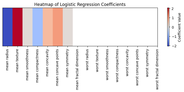
A heatmap (figure 5) provides insight into the importance and direction (positive or negative influence) of each principal component in the logistic regression model. The color intensity in the heatmap corresponds to the magnitude of the logistic regression coefficients. Warm colors (towards red) indicate positive coefficients, suggesting that as the value of the respective PC increases, the log-odds of the sample being benign also increase. Cool colors (towards blue) indicate negative coefficients, suggesting the opposite. For instance, PC1 (associated with mean radius) has a negative coefficient, implying that higher values of PC1 are associated with decreased odds of a tumor being benign.

Figure 5 (Heatmap of Logistic Regression Coefficients):

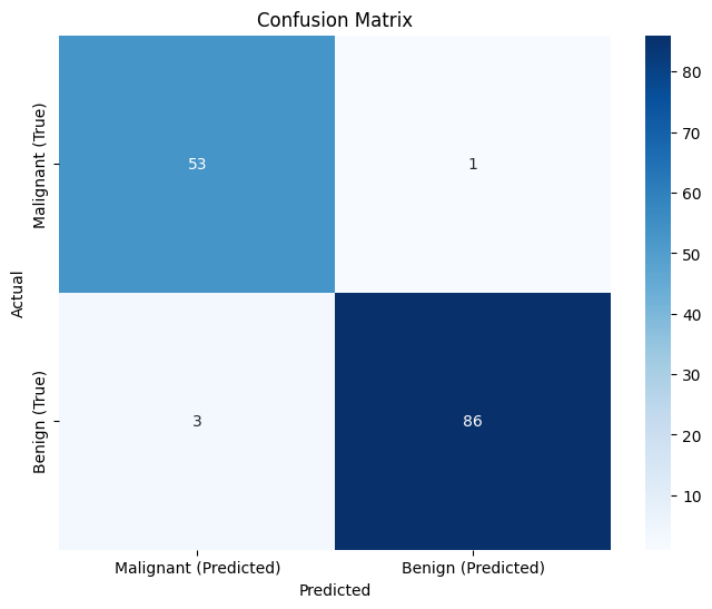
Finally, the confusion matrix in figure 6 summarizes the prediction results, showing the number of correct and incorrect classifications. The diagonal elements represent correctly classified samples (true positives and true negatives), while off-diagonal elements represent misclassifications (false positives and false negatives). In our matrix, the high values along the diagonal and the low values off the diagonal indicate that the model has a high accuracy and few misclassifications.

Figure 6 (Confusion Matrix):

Conclusion

This analysis utilized the Breast Cancer Wisconsin (Diagnostic) dataset to predict breast cancer diagnoses using logistic regression after addressing multicollinearity through feature selection and Principal Component Analysis (PCA). Feature selection involved eliminating the “error” variables, which reduced multicollinearity due to their close relationship with the “mean” variables. Two of the “radius,” “area,” and “perimeter” variables were eliminated, retaining only the “radius” variables, justified by their clinical utility in imaging reports. PCA was then employed to transform the data into uncorrelated principal components, capturing the most significant patterns while reducing dimensionality. The results from logistic regression on the PCA-transformed data showed an accuracy of 97.2%, with high precision and recall for both malignant and benign classes. The interpretation of the logistic regression coefficients in terms of odds ratios allowed for understanding the impact of each principal component on the likelihood of tumor malignancy. Visualization of the data projected onto the first two principal components demonstrated some separation between malignant and benign tumors but with some overlap, indicating the model’s ability to distinguish between the classes in a 2D space. Overall, the analysis successfully demonstrated the applicability of logistic regression and PCA in breast cancer diagnosis, highlighting the importance of feature selection and dimensionality reduction in enhancing the model’s performance and interpretability. These findings are crucial in contributing to the ongoing efforts to develop accurate and efficient diagnostic tools for breast cancer, potentially improving patient outcomes through earlier detection and intervention.